
Westend61/Getty Images
- You can use the IMPORTRANGE function in Google Sheets to easily copy data from one spreadsheet to another.
- To import data, you only need to know the URL and name of the original spreadsheet, and the range of cells to import.
- Once imported, the data is automatically updated when it changes in the original Google Sheets spreadsheet.
- Visit Insider's Tech Reference library for more stories.
If you work with Google Sheets often enough, you'll inevitably need to get data from one spreadsheet into another.
You could always simply copy and paste the cells in question, but if you do that, there's no live connection between the two sheets – if the original data changes, your second spreadsheet will become outdated.
Instead, you can use the IMPORTRANGE function, which quickly and easily helps you import data from one spreadsheet into another and keeps the two spreadsheets in sync at all times.
How to use IMPORTRANGE in Google Sheets
1. With only two arguments, using the IMPORTRANGE function is usually quite simple. Suppose you have a spreadsheet and you want to import the table into a new spreadsheet.
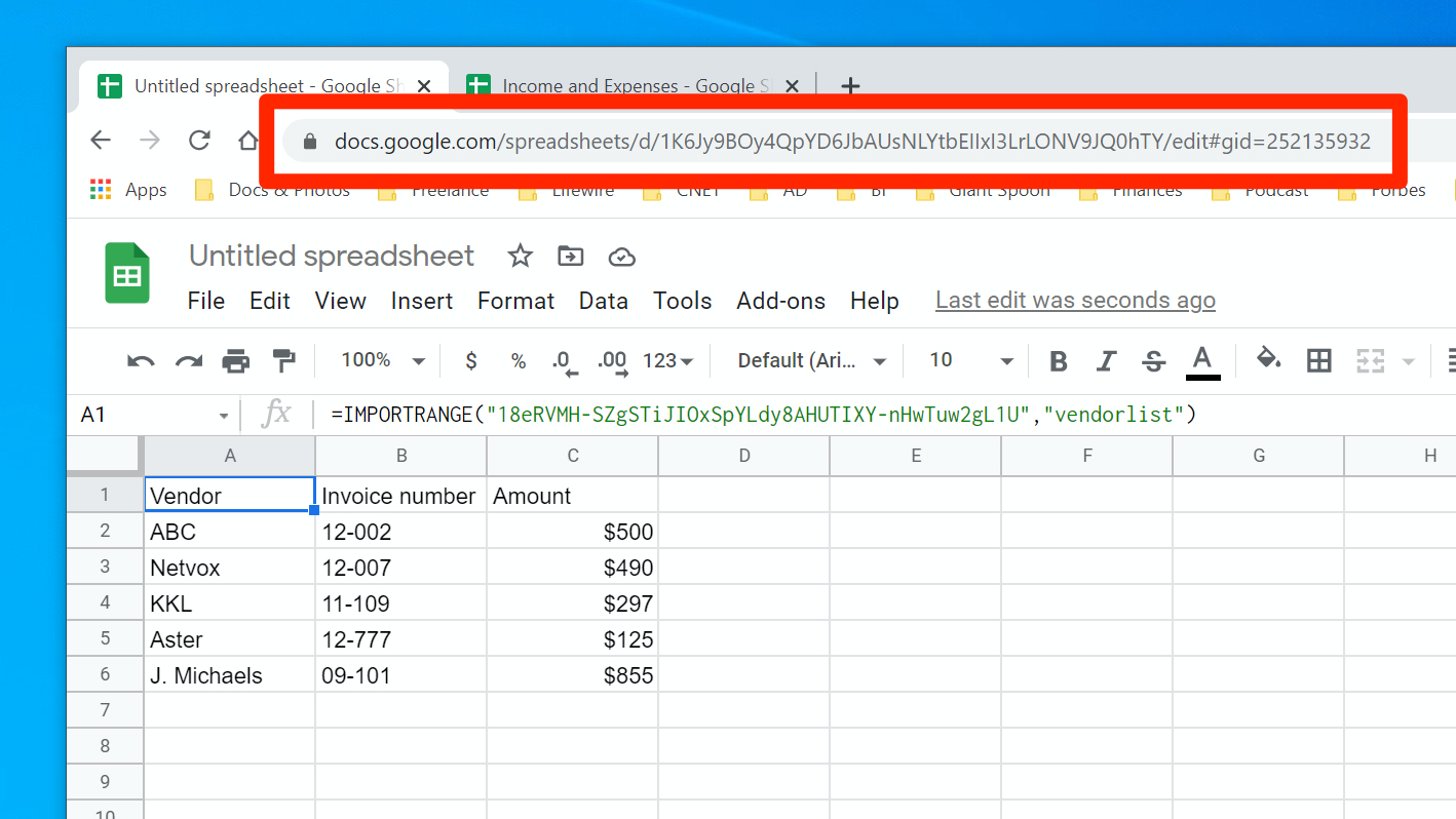
2. Click the URL in the address bar at the top of the browser and copy it. Alternately, you can copy just the spreadsheet key from within the URL.
Dave Johnson/Insider
3. In the new spreadsheet, type "=IMPORTRANGE(" - without the quotes.
4. Paste the URL and add a closing quote (").
5. Type a comma, add a quote (") and enter the range of cells you want to include. It should look like this: "Sheet1!B1:C6" Here, we're specifying that we want the spreadsheet named "Sheet1," and want cells B1 through C6.
6. Add a closing parenthesis and press Enter.
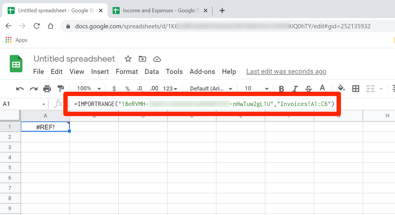
7. The complete function should look something like this:
=IMPORTRANGE("https://docs.google.com/spreadsheets/d/1Zoq0M0RG-RLYZ9HjOf01ff9eSPIYY3s/edit#gid=1027643093", "Sheet2!A1:C12")
Dave Johnson/Insider
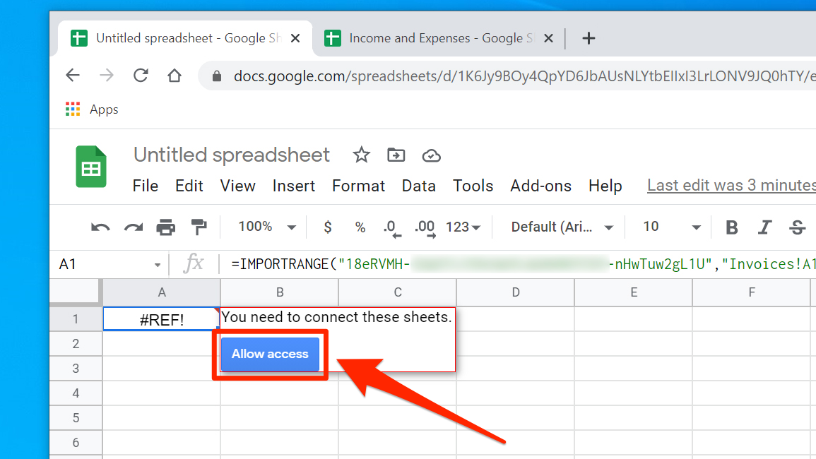
8. You might have noticed, though, that the data didn't import - there's a #REF! error in the cell instead. Click this cell and you'll see a message that you need to connect these sheets. Click "Allow access" and then, a moment later, the data should appear. You'll only need to do this once for each spreadsheet you import data from.
Dave Johnson/Insider
How to use the IMPORTRANGE function with a named range
If you prefer, you can use a named range instead of specifying the range in the manual way.
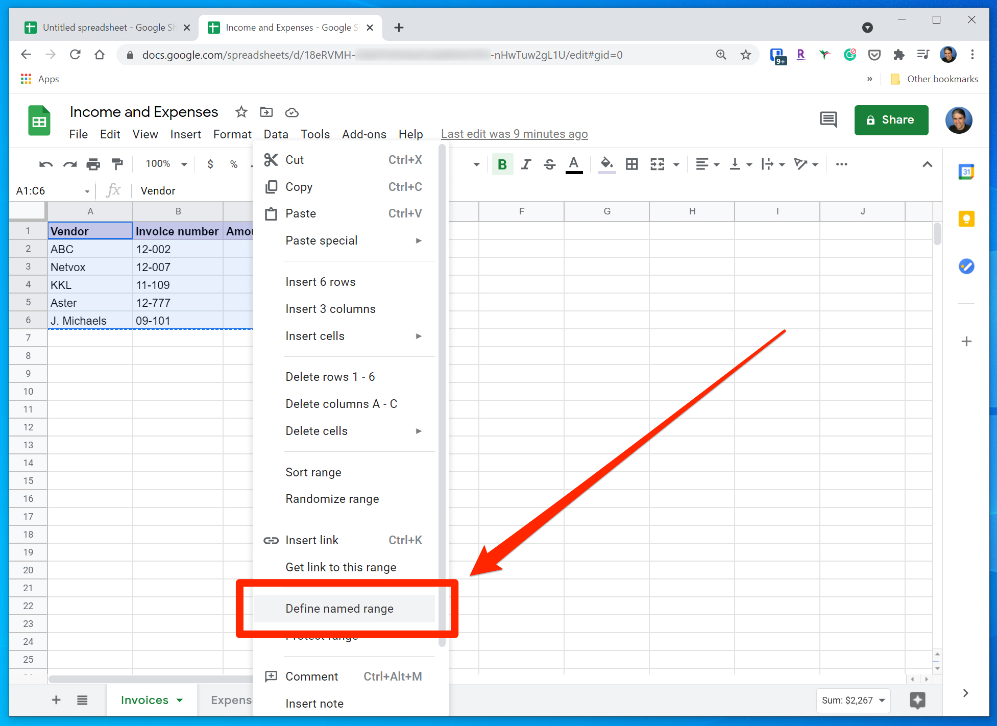
1. In the original spreadsheet, select the range and then right-click.
2. In the dropdown menu, choose "Define named range."
Dave Johnson/Insider
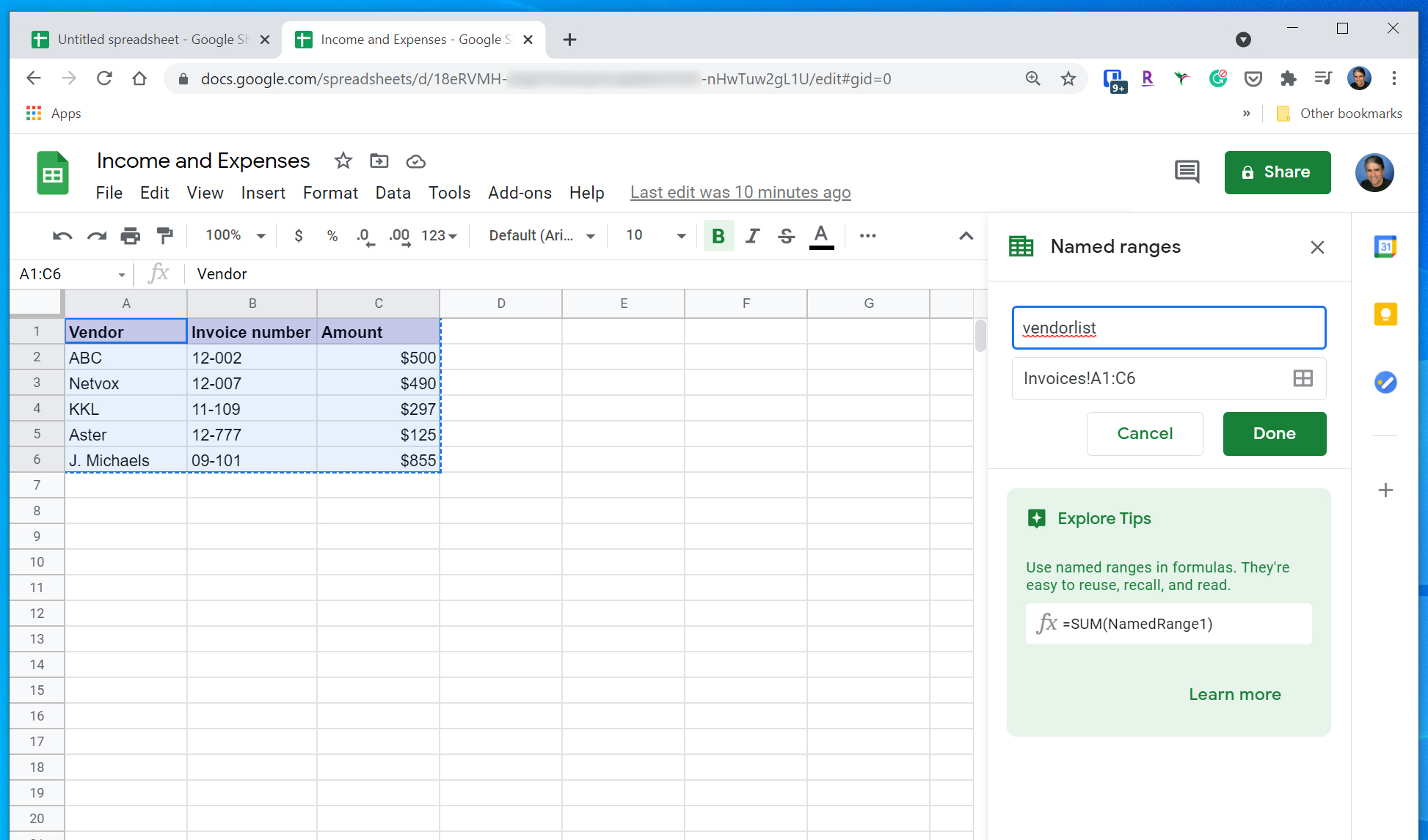
3. In the Named ranges pane that appears, give the selection a name and then click "Done."
Dave Johnson/Insider
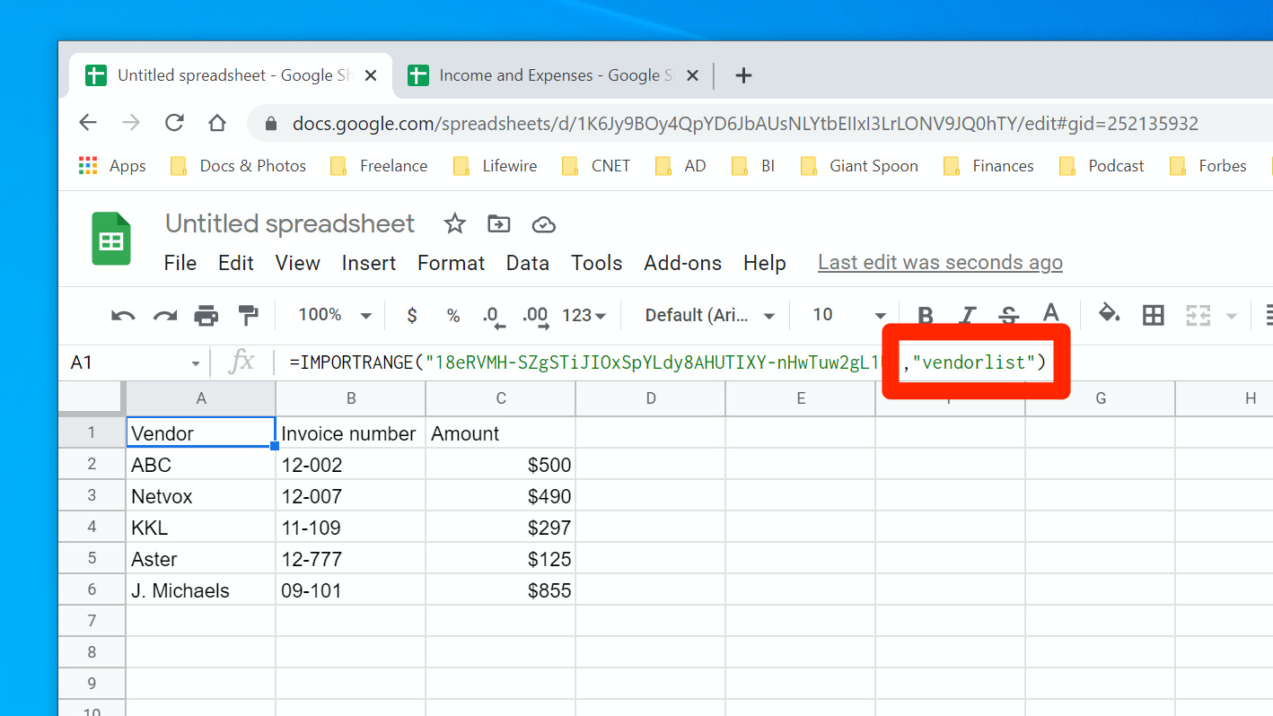
4. Now when you add your range_string to the IMPORTRANGE function, you can just enter this name, which already includes the name of the sheet. It's much easier than building the argument by hand.
Dave Johnson/Insider
Using the spreadsheet URL or spreadsheet key
There are a few nuances in the way this function works you should be aware of. Let's start with the URL.
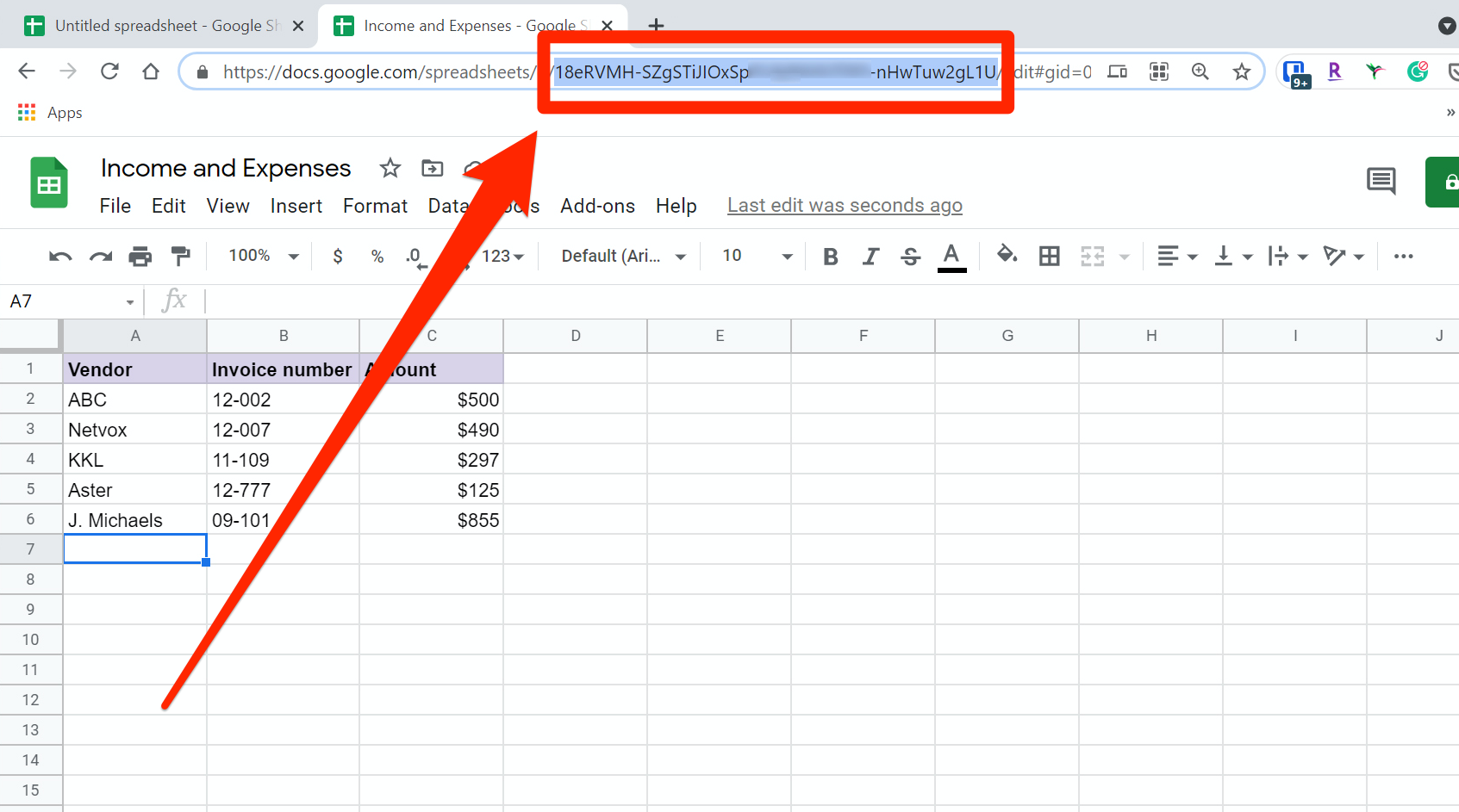
You have a choice: You can use the entire spreadsheet URL or you can use just the spreadsheet key, which is the part of the URL that follows the "d/." For example, suppose you had a spreadsheet with this URL:
https://docs.google.com/spreadsheets/d/1K6Jy9BAUsNLYtbEIIxI3LONV9JQ0hTY/edit#gid=25213
You can use the entire URL, or just the part after the d/:
1K6Jy9BAUsNLYtbEIIxI3LONV9JQ0hTY
Both options work exactly the same; the only difference is convenience, so use whichever works best for you. Either way, always enclose this argument in quotes.
Dave Johnson/Insider
Using the range_string
The range_string also has its own quirks. Specifically, when you enter the range in the IMPORTRANGE function, you need to clarify which sheet the cells are located in. Keep in mind that a spreadsheet might have many tabs, each being its own sheet. As a result, this argument takes this form:
Sheet1!A1:A12
In this example, Sheet1 is the name of the sheet, and the cells are indicated by the range A1:A12. You need to always include an exclamation mark between the sheet name and the range, and like the URL, always enclose it in quotes.
