cokada/Getty Images
- You can use the COUNTIF function in Google Sheets to find the number of items in a range that meet certain criteria.
- You can use text, numbers, and dates as criteria in the COUNTIF function.
- COUNTIF is an easy way to find out how many rows in a spreadsheet contain a blank cell, for example.
- Visit Insider's Tech Reference library for more stories.
Like Microsoft Excel, Google Sheets includes a simple COUNT function that tells you the number of items in the selected range. But what if you want to know the number of items based on some condition – like only the products in a list that are below a certain price, or only the cities in a specific state? That's when you would use the COUNTIF function.
As the name implies, COUNTIF combines the abilities of COUNT and IF – it checks to see if the IF argument is true before returning the COUNT value. Here's what the function looks like:
=COUNTIF(range, criterion)
- Range: This is the range of cells you want to test against some sort of criterion and then sum.
- Criterion: This is what you want to use to test against the range. You can use a number, text, or even a date as your criterion.
How to use COUNTIF in Google Sheets with a number condition
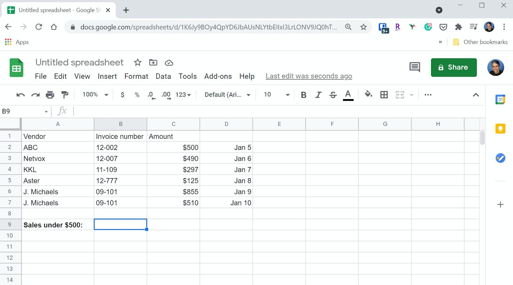
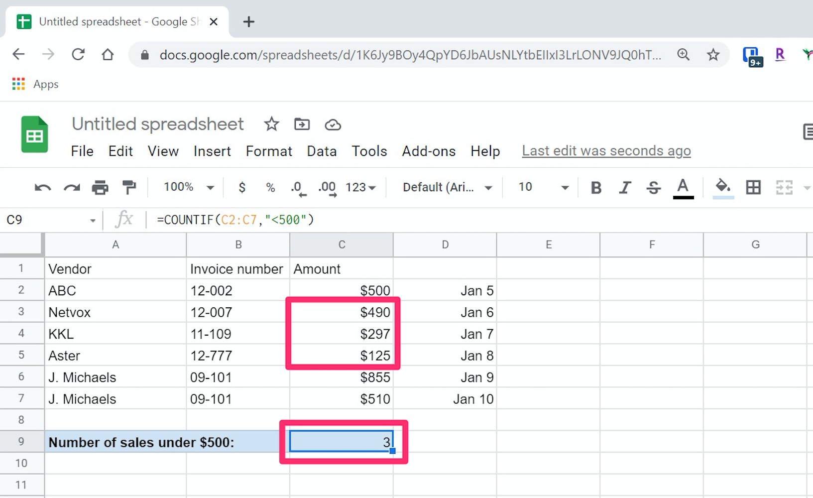
Using COUNTIF in your own Google Sheets is pretty straightforward, since you only need to specify two arguments. Suppose you had a spreadsheet like this in which you wanted to know how many items cost less than $500.

Dave Johnson/Insider
1. Type "COUNTIF" and press the Tab key. Google Sheets automatically adds the open parenthesis.
2. Click and drag the mouse to select the column that has the pricing information.
3. Type a comma and then enter the criteria - in this case "<500" (include the quotes).
4. Press the Tab key. Google Sheets will close the parenthesis and display the result in the cell.

Dave Johnson/Insider
How to use COUNTIF with a text condition
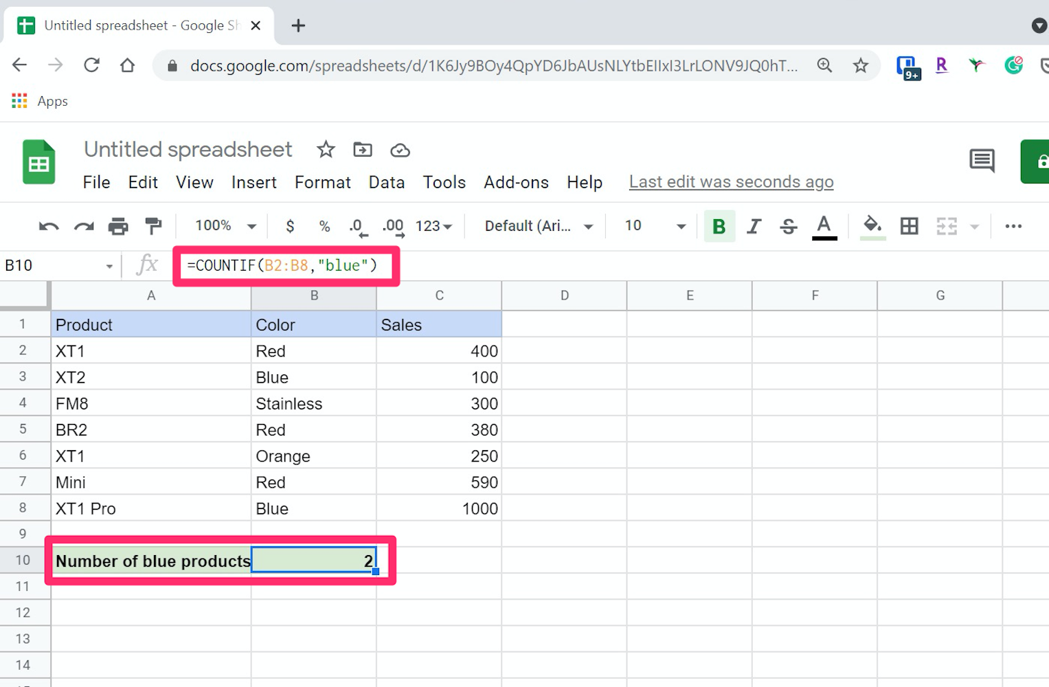
The COUNTIF function can also sum items based on text criteria. If you needed to find out how many items in a list have a particular color, you would do this:
1. Type "COUNTIF" and press the Tab key. Google Sheets automatically adds the open parenthesis.
2. Click and drag the mouse to select the column that has the color information.
3. Type a comma and then enter the criteria, such as "blue" (include the quotes).
4. Press the Tab key. You should see the result.

Dave Johnson/Insider
If you're looking for the sum of all the cells that don't have this value, that's easy to do as well - just use the NOT operator, like this:
=COUNTIF(A1:A12,"<>blue")
Likewise, the COUNTIF function is often used to find the number of entries that are blank, or the number that are not blank. This can be handy for cleaning up a messy spreadsheet. Find the blanks with a pair of quotes with nothing between:
=COUNTIF(A1:A12,"")
And the non-blank entries can be found with a NOT operator:
=COUNTIF(A1:A12,"<>")
How to use COUNTIF with a wildcard
Wildcards can come in handy because they help you find partial matches, such as all the descriptions that mention the color red.
1. Type "=COUNTIF" and press the Tab key.
2. Click and drag the mouse to select the column with the product descriptions.
3. Type a comma and then enter "*red*" (include the quotation marks).
4. Press the Tab key. Google Sheets will add the closing parenthesis and you should see the result in the cell.
In this example, we're looking for cells that contain the word red anywhere. But you could use "*red" to find cells that end with the word red or "red*" for cells that begin with red.
How to use COUNTIF with a date condition
The COUNTIF function can return the number of items that correspond to a particular date. Suppose we want to total all the sales that happened on January 15.
1. Type "=COUNTIF" and press the Tab key.
2. Click and drag the mouse to select the column with the range of dates.
3. Type a comma and then enter "DATE(2021, 1,15)" (do not include the quotation marks).
4. Press the Tab key. Google Sheets will add the closing parenthesis and you should see the result in the cell.
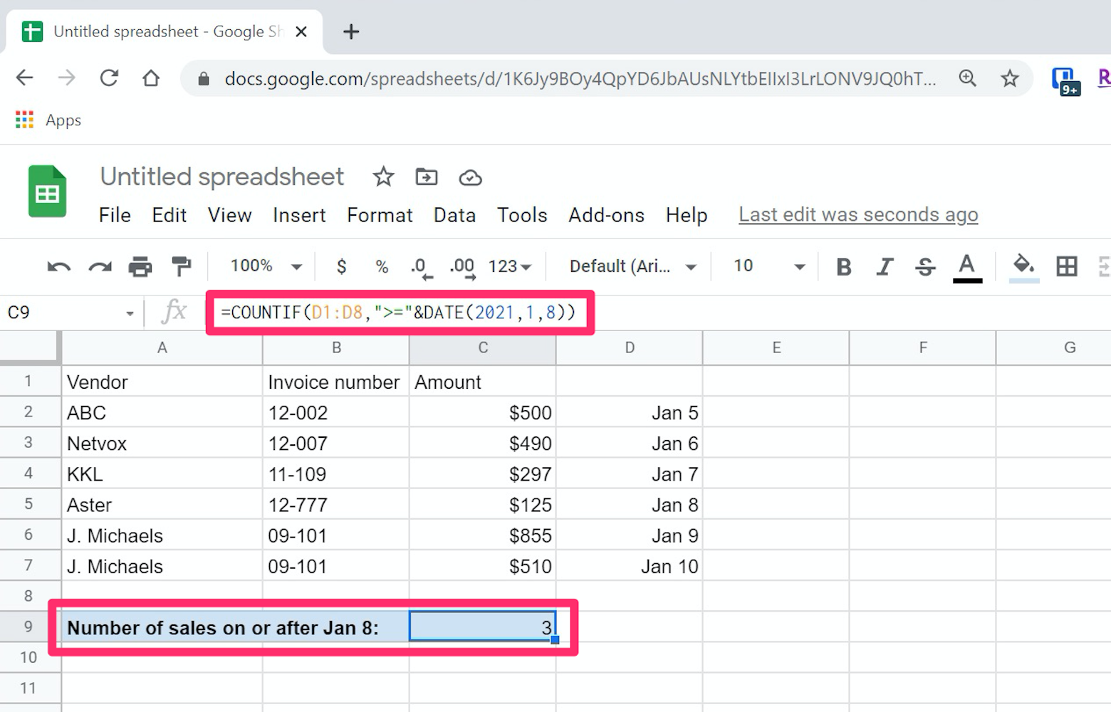
As you can probably guess, you can use variations of this argument with logical operators:
- =COUNTIF(D1:D8,">="&DATE(2021,1,7)). This returns the number of items dated on or after January 7.
- =COUNTIF(D1:D8,"<>"&DATE(2021,1,7)). This returns the number of items with any date other than January 7.

Dave Johnson/Insider
